Excel seating chart vs. Google Sheets: Which to choose?

Manually drawing a seating chart on paper is a one-time use. A digital classroom seating chart template Excel file, however, can be duplicated and adapted year after year.

You can create a functional seating chart in Excel in under an hour, even if you're not a power user. This guide will show you how to build one that's flexible enough to handle student absences, group changes, and even quick rearrangements for a special activity. We'll focus on a template that’s easy to update and visually clear, avoiding overly complex formulas unless absolutely necessary.

Setting Up Your Classroom Grid

First, let's visualize your classroom. Most teachers have a general idea of where desks are placed. We'll recreate this as a grid in your spreadsheet.

1. 01Open a new Excel workbook.
2. 02Define your grid dimensions. Imagine your classroom. If you have 5 rows of desks and 7 desks per row, you'll need a grid that’s at least 5 rows tall and 7 columns wide. We’ll add some buffer space for labels and spacing. Start by selecting a range of cells, say A1:G5, to represent your primary seating area.
3. 03Adjust row heights and column widths. To make it look like a classroom layout, select the rows (e.g., rows 1 through 5) and right-click to "Row Height." Enter a value like 30. Then, select the columns (e.g., columns A through G) and right-click to "Column Width." Enter a value like 10. This creates more uniform, square-like cells for your desks.
4. 04Add borders to delineate desks. Select the entire grid area (A1:G5 in our example). On the "Home" tab, in the "Font" group, click the "Borders" dropdown and choose "All Borders." This makes each cell look like an individual desk.

Adding Student Information

Now, let's populate these "desks" with student names. You have a few options here.

Option 1: Direct Entry

The simplest method is to type student names directly into the cells representing their desks.

1. 01Assign students to desks. Click into cell A1 and type the first student's name. Move to cell B1 for the next student, and so on. Continue filling across rows and then down to the next row.
2. 02Handle empty desks or absences. If a desk is empty or a student is absent, simply leave the cell blank or type "Absent."

Option 2: Using a Separate Student List

For larger classes or if you frequently rearrange students, it’s more efficient to have a separate list of your students and then "pull" their names into the seating chart. This is where a bit of Excel magic comes in handy.

1. 01Create a "Student List" sheet. Add a new sheet to your workbook by clicking the "+" button at the bottom. Rename this sheet "Student List."
2. 02List your students. In column A of the "Student List" sheet, starting from A1, enter all your students' names. In column B, you could add their student ID or any other relevant identifier.
3. 03Link names to the seating chart. Back on your main "Seating Chart" sheet, in the first desk cell (e.g., A1), you can use a formula to look up a student's name. If your student list is on the "Student List" sheet and their names are in column A, you could use a formula like =INDEX('Student List'!A:A, ROW(A1)). This formula will pull the first name from your student list into cell A1. You can then drag this formula across and down to fill your seating grid. If a student is absent, you can manually override the formula in the seating chart cell by typing "Absent" and then pressing Enter. Excel will ask if you want to replace the formula; say "Yes."

This method of linking is much faster if you need to completely reassign students. You would just reorder the names on your "Student List" sheet, and the seating chart would update automatically (unless you manually overrode cells).

Enhancing Visual Clarity with Formatting

A plain grid of names is functional, but we can make it much easier to read and use.

Conditional Formatting for Different Groups

Let's say you want to visually distinguish between students who are in "Group A" and "Group B."

1. 01Add a helper column. On your "Student List" sheet, add a new column (e.g., Column C) and label it "Group." Assign each student to a group (e.g., "A," "B," "C").
2. 02Apply conditional formatting. Go back to your "Seating Chart" sheet. Select the entire desk area (A1:G5).
3. 03Use the "New Rule" option. On the "Home" tab, in the "Styles" group, click "Conditional Formatting," then "New Rule."
4. 04Choose "Use a formula to determine which cells to format."
5. 05Enter the formula. If your formula in cell A1 on the seating chart is pulling a student's name from the "Student List" sheet using INDEX/ROW, you need to construct a formula that checks the group of that student. Assuming your INDEX/ROW formula in A1 is =INDEX('Student List'!A:A, ROW(A1)) and the group is in column C of the "Student List" sheet, the formula for conditional formatting would be:

=VLOOKUP(A1,'Student List'!A:C,3,FALSE)="A" (Note: This assumes you are directly typing names on the seating chart. If you're using the INDEX/ROW method to pull names, you’d need a slightly different approach or ensure the names in your seating chart match exactly those in the student list. A simpler approach is to have a column in your seating chart that looks up the group, and then apply conditional formatting to that column.)

Let’s refine this: On your "Seating Chart" sheet, next to your names, add a column (e.g., Column H) for "Group." In H1, you could put =VLOOKUP(A1,'Student List'!A:C,3,FALSE). Drag this down. Now, select your desk cells (A1:G5). Conditional Formatting Rule 1 (for Group A): Formula: =H1="A" Format: Set a fill color (e.g., light blue). Conditional Formatting Rule 2 (for Group B): Formula: =H1="B" Format: Set a different fill color (e.g., light green). Conditional Formatting Rule 3 (for Group C): Formula: =H1="C" Format: Set another fill color (e.g., light yellow).

Make sure the cell reference in the formula (e.g., H1) is the top-left cell of your selected range, and Excel will adjust it for the other cells.

Highlighting Specific Students

You might want to highlight students who need preferential seating or have specific needs.

1. 01Add another helper column on your "Student List" sheet, perhaps labeled "Notes."
2. 02Apply conditional formatting to your seating chart cells. Select the desk area.

Conditional Formatting Rule: Formula: =VLOOKUP(A1,'Student List'!A:D,4,FALSE)<>"" (This formula checks if there's any text in the "Notes" column for the student whose name is in A1). Format: Set a distinct border or fill color (e.g., a red border).

Adding Room Features

Your classroom isn't just a grid of desks. You have a door, a whiteboard, and maybe some windows or cabinets.

1. 01Use merged cells to represent larger features. For example, to represent a whiteboard at the front of the room, select a range of cells across the top row (e.g., C1:E1) and click "Merge & Center" on the "Home" tab. Type "Whiteboard" into the merged cell.
2. 02Use cell colors to denote other areas. You can color cells or groups of cells to represent the door, teacher's desk area, or reading corner. Select the cells, and use the "Fill Color" option from the "Font" group on the "Home" tab.

Practical Considerations and Tips

When building your classroom seating chart template Excel file, keep these points in mind:

• Student IDs vs. Names: For privacy, especially if you share printouts, using Student IDs might be preferable. You can then have a separate, secure list of IDs to names.
• Printability: If you plan to print the chart, ensure the "Page Layout" settings (orientation, scaling) are adjusted so it fits on a single page. You might need to reduce font sizes or the overall grid size.
• Flexibility for Activities: For special activities, you might want to create duplicate sheets within the same workbook. Just right-click the sheet tab, choose "Move or Copy," check "Create a copy," and click "OK." You can then rename this new sheet "Activity Seating" and rearrange students as needed.
• Saving as a Template: Once you're happy with your design, save the file as an Excel Template (.xltx). Go to "File" > "Save As," choose a location, and in the "Save as type" dropdown, select "Excel Template." This way, whenever you open the file, you'll get a new, unsaved copy, preserving your original template.

Common Mistakes to Avoid

• Over-complicating Formulas: Resist the urge to use extremely complex nested formulas. Simple VLOOKUP or INDEX/MATCH for pulling data is usually sufficient. If your needs go beyond that, consider if Excel is still the best tool or if a dedicated school management system is more appropriate.
• Not Planning for Absences: Always leave room or a clear method for indicating when a student is out. A blank cell is fine, but a dedicated "Absent" entry can be clearer.
• Forgetting to Update: The best seating chart is useless if it's not current. Make it a habit to review and update it regularly, especially after student withdrawals or additions.
• Making it Unreadable: Too many colors, too small a font, or a cluttered layout will defeat the purpose. Prioritize clarity and ease of reading.

Frequently Asked Questions

How do I make my classroom seating chart look professional?

Use consistent formatting. Stick to one or two clear fonts, use borders strategically to define desks and sections, and employ a limited, purposeful color palette for visual cues like group assignments. Ensure row heights and column widths are uniform for a clean, grid-like appearance.

Can I use this for different class sizes?

Yes, by adjusting the number of rows and columns. If you have a smaller class, you can simply use a portion of the grid and leave the rest blank, or hide unused rows and columns. For larger classes, you might need to expand the grid or create multiple charts. The template structure allows for easy resizing.

What if I have students who need to sit near the front or away from distractions?

You can use conditional formatting or simply add a note in a helper column for those students. When you're arranging students, you can filter your student list by these criteria or visually scan for highlighted students to ensure their needs are met during the manual placement process. For more complex behavioral tracking, a Behavioural Chart might offer deeper insights.

Is there a way to track student behavior alongside their seating?

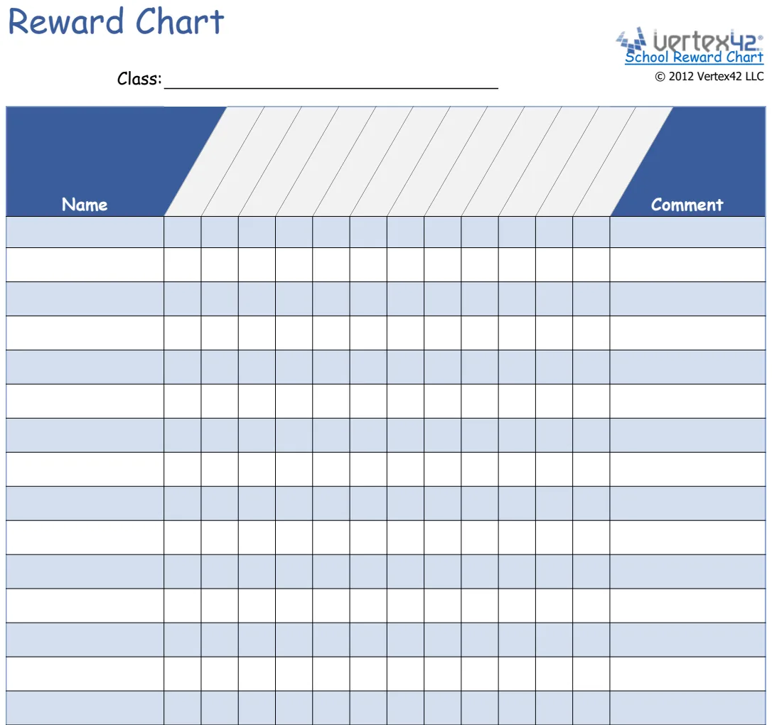
While a seating chart primarily focuses on physical location, you could integrate a simplified behavior note if you have a small class. For systematic behavior tracking, however, dedicated tools are far more effective. You might find a School Reward Chart useful for positive reinforcement, or a School Reward Chart to manage broader classroom rewards.