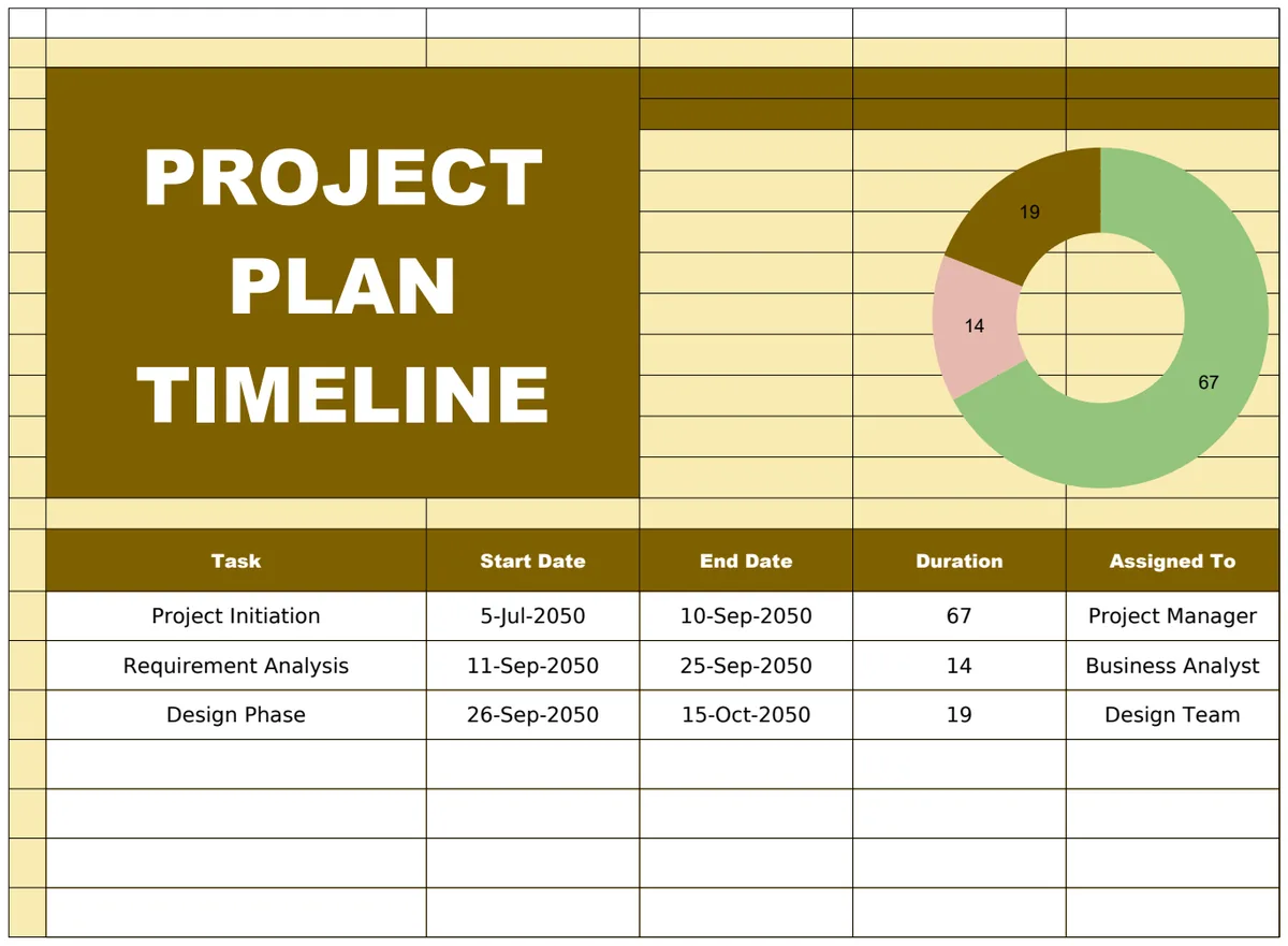
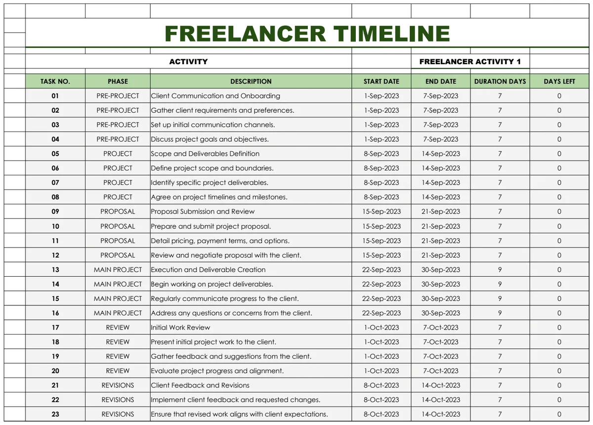
A stakeholder asks one question: "When does this land, and what has to happen first?" You have the answer in a spreadsheet, spread over 40 rows of dates and names, and nobody can read it at a glance. A timeline fixes that. It turns a list of dates into a picture people understand in five seconds, which is why it ends up on status reports, launch plans and slide decks.
Excel does not have a built-in timeline chart, so most people either draw one by hand with shapes or give up. There are better ways. This guide covers three methods, from the quick one to the one that redraws itself when a date changes, with the formulas for workdays, dependencies and a "today" marker. It also covers the difference between a timeline and a Gantt chart, because the two get mixed up all the time.
Timeline vs Gantt chart
They answer different questions, and a good project plan usually needs both.
- A timeline shows key dates: milestones, events and deadlines along a line. It is best for communicating, such as an executive summary or a customer-facing roadmap.
- A Gantt chart shows tasks as bars with a start, an end and progress. It is best for managing: who is doing what, what overlaps and what is late.
A timeline is the headline and a Gantt chart is the detail. If you keep both in one list of items, the timeline never contradicts the plan underneath it.
Method 1: a SmartArt timeline (fastest, but manual)
Excel includes a ready-made graphic:
- 01Go to Insert, then SmartArt.
- 02Choose Process, then Basic Timeline.
- 03Type your milestones into the text pane.
It takes two minutes and looks neat for a handful of items. The catch is that SmartArt knows nothing about dates. The spacing between milestones is the same whether they are a week apart or a year apart, and nothing moves when a date changes. Use it for a simple five-step overview, not for a real plan.
Method 2: a scatter chart that places items by date
This is the method that gives you a true timeline, because the horizontal position comes from the actual date. It needs a little setup, and then it updates itself.
Step 1: set up a clean list
Create columns for Item, Date, Category and Owner. Make sure the dates are real dates, not text. A quick check: =ISNUMBER(B2) should return TRUE. Excel stores dates as serial numbers, so 4 January 2027 is 46391, and that number is what the chart plots.
Step 2: add a height column
Labels collide if every item sits on the same line. Give each item a height above or below the axis. A simple formula alternates above and below and cycles through three heights:
=IF(ISODD(n), 1, -1) * (1 + MOD(n-1, 3))
Here n is the item number. Item 1 goes above at height 1, item 2 below at height 2, item 3 above at height 3, item 4 below at height 1, and so on. Three levels is usually enough to keep labels from overlapping.
Step 3: insert the chart
- 01Select the Date column and the Height column.
- 02Insert, then Scatter, then Scatter with only markers.
- 03Format the axis: set the minimum and maximum to your first and last dates and hide the vertical axis.
Step 4: add stems and labels
- Stems: add Y error bars with a Minus direction and a 100 percent value, so each marker has a line down to the axis.
- Labels: select the series, add Data Labels, then choose "Value From Cells" and point it at your Item column. This option exists in Excel 2013 and later.
Step 5: colour by category
A single series has one colour. To colour by category, make one series per category, each with its own height column that shows NA() unless the item belongs to it:
=IF($C2="Design", $D2, NA())
NA() is deliberate here. Excel skips #N/A points in a chart, so only the items in that category are drawn. Keep these helper columns off to the side, or hide them, so the #N/A values never show up in the main sheet.
Step 6: draw a today line
Add a two-point series with the x value =TODAY() at the top and bottom of the chart's height range, and format it as a dashed line. It moves every day without any editing.
Method 3: a Gantt chart from a stacked bar chart
For tasks with durations, use a stacked bar chart:
- 01Create columns for Task, Start and Duration (in days).
- 02Select Task, Start and Duration and insert a Stacked Bar chart.
- 03Click the Start series and set its fill to None, so only the duration bars show.
- 04Format the vertical axis and tick "Categories in reverse order" so the first task sits at the top.
- 05Set the horizontal axis minimum to the project start date's serial number, 46391 in our example below.
To show progress, split the bar into two series: done =Duration * PercentComplete and remaining =Duration * (1 - PercentComplete), with different colours.
Dates that update themselves: workdays and dependencies
A timeline that is correct on Monday and wrong on Friday is worse than none. Make the dates calculate.
End date from a duration in workdays:
=WORKDAY(Start, Duration - 1, Holidays)
Holidays is a named list of dates the calculation should skip, along with weekends. The minus one matters: a 10-day task that starts on Monday ends on the second Friday, not the Monday after.
Start date from a predecessor:
=WORKDAY(PredecessorEnd, 1, Holidays)
Workdays between two dates:
=NETWORKDAYS(Start, End, Holidays)
Status from a status date:
=IF(Pct=1, "Done", IF(End < StatusDate, "Late", IF(Start <= StatusDate, "In progress", "Not started")))
Using a status date cell instead of TODAY() keeps last week's report from changing when you reopen it.
A worked example: a launch plan that moves when something slips
A fictional app launch starts on Monday 4 January 2027, with one company holiday on 15 February. Each task starts the next workday after the one before it ends.
| Task | Workdays | Start | End |
|---|---|---|---|
| Research | 10 | Mon 4 Jan | Fri 15 Jan |
| Design | 15 | Mon 18 Jan | Fri 5 Feb |
| Build | 30 | Mon 8 Feb | Mon 22 Mar |
| Testing | 10 | Tue 23 Mar | Mon 5 Apr |
| Launch (milestone) | n/a | Tue 6 Apr | Tue 6 Apr |
The whole plan runs 92 calendar days, from 4 January to the 6 April launch.
Now design runs five workdays over, so it takes 20 days and ends on Friday 12 February. Because every later task depends on the one before it:
- Build now starts Tue 16 Feb, since 15 February is a holiday, and ends Mon 29 Mar.
- Testing runs from Tue 30 Mar to Mon 12 Apr.
- Launch moves from 6 April to 13 April.
Five workdays of slip became a launch seven calendar days later. Nobody had to edit the later rows by hand, and that is what the WORKDAY formulas buy you. If the dates are typed in, someone will forget to move one.
History and event timelines
Timelines are not only for projects. Teachers, researchers and content teams use them for history, product releases and campaigns. The same scatter method works, with two limits:
- Excel dates begin on 1 January 1900, so earlier dates cannot be plotted. For ancient history, use a year number such as -500 or 1066 as a plain number on the axis instead of a date.
- Rename the categories to eras, themes or regions and leave the owner blank.
Mistakes that ruin Excel timelines
- Dates stored as text. They look right and plot wrong. Test with
ISNUMBER. - Typing end dates. Use durations and workday formulas so changes flow through.
- Everything at one height. Labels overlap and the chart becomes unreadable. Use staggered heights.
- A fixed axis. If the axis does not follow your dates, new items fall off the chart. Link the minimum and maximum to the first and last date, or to a zoom window.
- Too many milestones. Past 20 or so, a timeline becomes a wall of text. Show the important ones and keep the rest on the Gantt chart.
- A today line you typed in. Use
TODAY()or a status date. - Showing helper columns. Hide them, or the
#N/Avalues will confuse the next person.
A timeline that draws itself
Building the scatter method once is satisfying, and rebuilding it for every project is not. The Project Timeline & Milestone Maker turns a simple list into a finished timeline chart. Add each milestone or event with its date and category on the Plan tab, and it appears on the Timeline, alternating above and below the axis at three heights so labels do not overlap.
Each category has its own colour and a dashed line marks today. Axis labels switch between weeks, months, quarters and years, and you can zoom by typing a window start and end on Settings. The Timeline prints on one landscape page with a table of the items shown, which makes it ready for a status report or a slide.
Tasks carry a start date and an end date or a duration in workdays. Weekends and your listed holidays are skipped, and a task that depends on an earlier item starts the next working day after it finishes, so when something slips the work after it moves too. The Gantt tab shows every task as a bar shaded by percent complete, with late work in red, milestones as diamonds and today's column highlighted. The Dashboard shows progress weighted by workdays, milestones hit, late items with days overdue, items due soon and open work by owner. It holds 100 items, with the first 24 in the chosen window plotted on the timeline chart, locks the formulas without a password and contains no macros.
If you only need part of it, these templates may be enough:
Common questions
How do I create a timeline in Excel?
For a quick overview, use Insert, SmartArt, Process, Basic Timeline. For a timeline that places items by their real dates, build a scatter chart with the date on the x axis and a height column on the y axis, then add error bars as stems and labels from cells. A template can do all of that for you from a simple list.
What is the difference between a timeline and a Gantt chart?
A timeline shows key dates, such as milestones and events, at a glance. A Gantt chart shows tasks as bars with their start, end and progress. Most projects benefit from both, built from the same list.
How do I make an Excel timeline update automatically?
Use real dates, calculate end dates with WORKDAY from a duration, start dependent tasks with WORKDAY from the previous task's end, and base the chart on cells rather than on typed numbers. Then a changed date moves everything after it.
Can I make a timeline for dates before 1900?
Not with Excel dates, which start in 1900. For history timelines, use years as plain numbers and format the axis accordingly.
How do I add a today line to an Excel timeline?
Add a series with two points at the x value =TODAY(), one at the top and one at the bottom of the chart, and format it as a dashed line.
Does it work in Google Sheets?
The workbook is built for Microsoft Excel 2016 or later (desktop or Excel for the web). You can import it into Google Sheets, but sheet protection does not carry over, and Google Sheets draws charts differently, so the timeline chart may not look the same.
A timeline you can read in five seconds saves a lot of status meetings. You can preview the Project Timeline & Milestone Maker free; downloading it is included in the OpenWorksheet monthly plan, along with the rest of the library. The dates in this guide are examples for a fictional project.